Filtering genes
I was playing with GTEx v8 data, so I first filtered lowly-expressed genes after some prepossesses:
library(edgeR)
tissue.no <- pData(eset) %>%
             group_by(SMTSD) %>%
             summarise(n=n())

# in tissue-aware manner, refer to YARN paper
min(tissue.no$n) #113
minSamples <- floor(min(tissue.no$n)/2)
cnt.cpm <- cpm(exprs(eset))
keep <- rowSums(cnt.cpm > 1) >= minSamples
eset <- eset[keep,]
dim(eset)
## Features  Samples
##    29212    14437
Normalization comparisons
Normalize selected samples in tissue-aware way.
- TMM: trimmed mean of M-values
- RLE: relative log expression
- UQ: upper quartile
- DESeq: median-ratio-scaling
- QN: quantile normalization
- qsmooth: smooth quantile normalization
- none: original data
The following is a simple function to perform all of these, extended the one in yarn.
## tissue aware normalization, all returing log2-transformed cpm since limma uses cpm
tissue.aware.norm <- function(eset, group, method=c('TMM', 'RLE', 'UQ', 'DESeq', 'QN', 'qsmooth', 'none'), logOutput=TRUE) {
  suppressPackageStartupMessages({
    library(edgeR)
    library(doParallel)
    library(preprocessCore)
    library(DESeq2)
    library(qsmooth)
  })
  if (length(group) == 1) tissues <- factor(pData(eset)[, group])

  # function to retrieve normalized counts from dge list
  getDGEcnts <- function (dge) {
    dge <- estimateCommonDisp(dge)
    dge <- estimateTagwiseDisp(dge)
    norm.cnts <- t(t(dge$pseudo.counts)*(dge$samples$norm.factors))
    norm.cnts
  }

  if (method == 'TMM') {
    # weights are from the delta method on Binomial data
    normalizedMatrix <- foreach(tissue = unique(tissues), .combine = cbind) %dopar% {
      cnts <- exprs(eset[, which(pData(eset)[, group] %in% tissue)])
      dge <- DGEList(cnts)
      dge <- calcNormFactors(dge, method = 'TMM')
      norm.cnts <- getDGEcnts(dge)
      norm.cnts
    }
  } else if (method == 'RLE') {
    # the median ratio of each sample to the median library (geometric mean of all columns) is taken as the scale factor
    normalizedMatrix <- foreach(tissue = unique(tissues), .combine = cbind) %dopar% {
      cnts <- exprs(eset[, which(pData(eset)[, group] %in% tissue)])
      dge <- DGEList(cnts)
      dge <- calcNormFactors(dge, method = 'RLE')
      norm.cnts <- getDGEcnts(dge)
      norm.cnts
    }
  } else if (method == 'UQ') {
    # the scale factors are calculated from the 75% quantile of the counts for each library
    normalizedMatrix <- foreach(tissue = unique(tissues), .combine = cbind) %dopar% {
      cnts <- exprs(eset[, which(pData(eset)[, group] %in% tissue)])
      dge <- DGEList(cnts)
      dge <- calcNormFactors(dge, method = 'upperquartile')
      norm.cnts <- getDGEcnts(dge)
      norm.cnts
    }
  } else if (method == 'none') {
    # scale factors are 1
    normalizedMatrix <- foreach(tissue = unique(tissues), .combine = cbind) %dopar% {
      cnts <- exprs(eset[, which(pData(eset)[, group] %in% tissue)])
      dge <- DGEList(cnts)
      dge <- calcNormFactors(dge, method = 'none')
      norm.cnts <- getDGEcnts(dge)
      norm.cnts
    }
  } else if (method == 'DESeq') {
    # counts divided by median ratio of gene counts relative to geometric mean per gene
    normalizedMatrix <- foreach(tissue = unique(tissues), .combine = cbind) %dopar% {
      cnts <- exprs(eset[, which(pData(eset)[, group] %in% tissue)])
      dds <- DESeqDataSetFromMatrix(countData = cnts, colData = pData(eset[, which(pData(eset)[, group] %in% tissue)]), design = ~ 1)
      dds <- estimateSizeFactors(dds)
      #cpm <- fpm(dds, robust = T) #a robust method using specific library sizes
      norm.cnts <- counts(dds, normalized=T)
      norm.cnts
    }
  } else if (method == 'QN') {
    normalizedMatrix <- foreach(tissue = unique(tissues), .combine = cbind) %dopar% {
      cnts <- exprs(eset[, which(pData(eset)[, group] %in% tissue)])
      norm.cnts <- normalize.quantiles(cnts, copy=F)
      norm.cnts
    }
  } else if (method == 'qsmooth') {
    exprs <- exprs(eset)
    qs <- qsmooth(exprs, group_factor = tissues)
    normalizedMatrix <- qsmoothData(qs)
  } else {
    stop('YEEEE... code it by yourself if you wanna do it.')
  }

  if (logOutput) {
    normalizedMatrix <- log2(normalizedMatrix + 1)
  }
  normalizedMatrix <- normalizedMatrix[, match(rownames(pData(eset)), colnames(normalizedMatrix))]
  normalizedMatrix
}
Visualizing distributions
I picked some tissues to see their distribution.
Some helper functions:
getColors <- function(vec) {
  # assgin a color to each group of samples
  library(RColorBrewer)
  n <- length(unique(vec))
  col <- brewer.pal(n, "Paired")
  #col <- brewer.pal.info[brewer.pal.info$category=='qual', ] # get max. 74 colours
  #col_all <- unlist(mapply(brewer.pal, col$maxcolors, rownames(col)))
  ifelse (n > length(col),
          cvec <- sample(col, n, replace=T),
          cvec <- sample(col, n, replace=F)
  )
  vec <- as.character(vec)
  names(vec) <- rep(NA, length(vec))
  for (g in 1:length(unique(vec))) {
    names(vec)[which(vec==unique(vec)[g])] <- cvec[g]
  }
  vec
}


dens.plot <- function(table, colVec, ...) {
  cols <- names(colVec)
  d <- plot(density(table[, 1]), col=cols[1],
            lwd=2, las=2, xlab="", ...) +
    abline(v=0, lty=3) + title(xlab="log2 exprs", ylab=NA) +
    for (i in 2:ncol(table)) {
      den <- density(table[, i])
      lines(den$x, den$y, col=cols[i], lwd=2)
    }
  legend('topright', legend=unique(colVector), lty=1, col=unique(names(colVector)), cex=0.6)
  d
}
Plot distributions:
selectt <- c('Brain - Amygdala', 'Artery - Aorta', 'Heart - Atrial Appendage', 'Whole Blood', 'Testis')
sub.eset <- eset[, which(pData(eset)$SMTSD %in% selectt)]
dim(sub.eset)

dist.list <- list()
methods <- c('TMM', 'RLE', 'UQ', 'DESeq', 'QN', 'qsmooth', 'none')
for (n in methods) {
  dist.list[[n]] <- tissue.aware.norm(sub.eset, "SMTSD", n)
}
#saveRDS(dist.list, file='~/cvd/v8/exprs/norm.cpm.rds')

sub.p <- pData(sub.eset)
sub.p$SMTSD <- factor(sub.p$SMTSD)
sub.p <- sub.p[order(sub.p$SMTSD),]
colVector <- getColors(sub.p$SMTSD)

mypar(3, 3)
for (n in methods) {
  print(dens.plot(dist.list[[n]][,match(rownames(sub.p), colnames(dist.list[[n]]))], colVector, ylim=c(0, 0.3), main=n))
}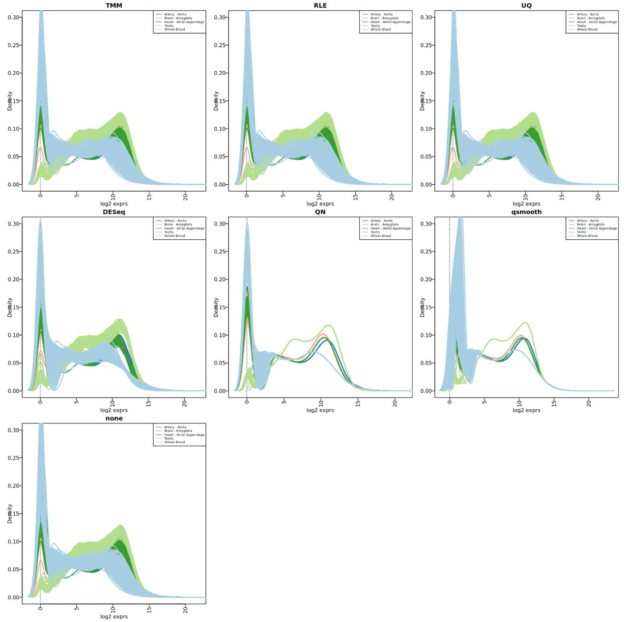
Seems there are still many lowly-expressed genes in some of these tissues, testis looks good though. The first three - TMM, RLE, UQ - are quite similar; DESeq method seems the same as none.